Option Pricing When a Single Jump is Anticipated II - Matthias Thul's HomepageMatthias Thul's Homepage

In this post, I augment a constant coefficient geometric Brownian motion process by a single jump whose time of occurrence is known. The random variable representing the jump size follows a normal mixture distribution. To get a feeling for the impact of predictable jumps on option prices, we inspect the shape of a few model implied probability densities and volatility smiles.

Jump Size Distribution

Using the previously introduced notation, we model the jump size $Y$ to follow a mixture of $n$ independent normal random variables $\left\{ Z_i \right\}_{i = 1}^n$ with $Z_i \sim \mathcal{N} \left( \mu_i, \sigma_i^2 \right)$ . It has the probability density and characteristic function

$\begin{eqnarray*} f_Y(x) & = & \sum_{i = 1}^n p_i \frac{1}{\sqrt{2 \pi} \sigma_i} \exp \left\{ -\frac{\left( x - \mu_i \right)^2}{2 \sigma_i^2} \right\},\\ \phi_Y(\omega) & = & \sum_{i = 1}^n p_i \exp \left\{ \mathrm{i} \mu_i \omega - \frac{1}{2} \sigma_i^2 \omega^2 \right\} \end{eqnarray*}$

where $p_i \in [0, 1]$ are the weights satisfying $\sum_{i = 1}^n p_i = 1$ .

Implied Volatility Smiles

We now consider a few implied volatility smiles implied by the above jump size distribution and when $n = 2$ . The base dynamics follow a constant coefficient geometric Brownian motion with $\sigma = 15\%$ . The jump time is in 1 calendar day and we value European plain vanilla options with a common maturity of 7 calendar days.

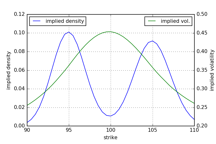
The first example below shows the implied probability density and volatility smile for $p_1 = p_2 = 50\%$ , $\mu_1 = +5\%$ , $\mu_2 = -5\%$ and $\sigma_1 = \sigma_2 = 0.0\%$ . I.e. with equal probability there is a point jump up or down with an absolute jump return of $5\%$ . The resulting implied probability density is bi-modal with a mode at each of the two mean jump returns. We notice that the implied volatility smile is concave near-the-money which indicates that the corresponding implied density is platykurtic, i.e. has a negative excess kurtosis. As this example illustrates, such a situation is not necessarily a violation of static no-arbitrage conditions.

Consider now what happens when we change $\mu_1 = +10\%$ and $\mu_2 = 0\%$ . I.e. either there is a significant up-jump or nothing happens. It turns out that the corresponding plot looks identical to the previous one. The reason for this is that the jump drift compensator in

$\begin{equation*} \gamma(t) = r - \frac{1}{2} \sigma^2 - \ln \left( \phi_Y(-\mathrm{i}) \right) \delta \left( t - t_J \right) \end{equation*}$

ensures that the expected jump return is always zero. This has to be the case in the risk-neutral dynamics as the model would otherwise allow for an expected instantaneous profit.

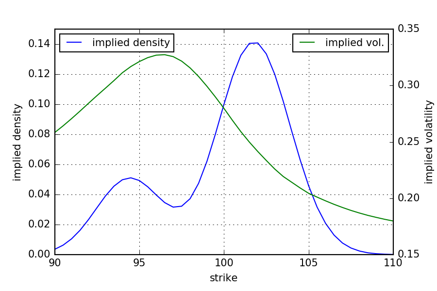
We now consider an asymmetric case like it is often observed in real markets. There is a positive jump with a relative probability $p = 75\%$ but low return $\mu_1 = 2.5\%$ . The negative jump on the other side has a low probability but high absolute return $\mu_2 = -5\%$ . We again consider the special case of point jump with zero standard deviation. The implied volatility smile is still concave though the mode now shifted to the downside and the upper tail decays faster due to the smaller positive jump return.

Leave a Reply Cancel reply