Automatic (Differentiation) for the COS Method - Matthias Thul's HomepageMatthias Thul's Homepage

In the last post, I provided a brief introduction to forward mode automatic differentiation with CppAD. In this post, I propose to use automatic differentiation for the computation of cumulants of option pricing models based on characteristic functions. This is useful, for example, when pricing European vanilla options using the Fang and Oosterlee (2008) COS method. Here, the first four cumulants are used to determine the integration range.

Cumulants

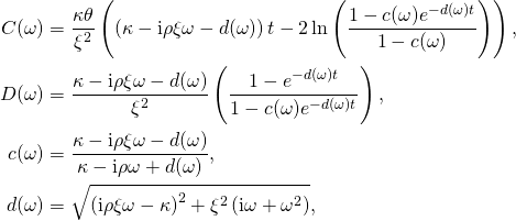
While analytical expressions for the cumulants can usually be obtained with the help of some computer algebra system, they can easily become very long. Consider for example the characteristic function for the Heston (1993) stochastic volatility model. The cumulant generating function of the martingale component is

$\psi_t^{\text{SV}}(\omega) = C(\omega, t) + D(\omega, t) V_0, \nonumber$

where

$\begin{align*} C(\omega) & = \frac{\kappa \theta}{\xi^2} \left( \left( \kappa - \mathrm{i} \rho \xi \omega - d(\omega) \right) t - 2 \ln \left( \frac{1 - c(\omega) e^{-d(\omega) t}}{1 - c(\omega)} \right) \right),\\ D(\omega) & = \frac{\kappa - \mathrm{i} \rho \xi \omega - d(\omega)}{\xi^2} \left( \frac{1 - e^{-d(\omega) t}}{1 - c(\omega) e^{-d(\omega) t}} \right),\\ c(\omega) & = \frac{\kappa - \mathrm{i} \rho \xi \omega - d(\omega)}{\kappa - \mathrm{i} \rho \omega + d(\omega)},\\ d(\omega) & = \sqrt{\left( \mathrm{i} \rho \xi \omega - \kappa \right)^2 + \xi^2 \left( \mathrm{i} \omega + \omega^2 \right)}, \end{align*}$

see e.g. Albrecher et al. (2007). The second cumulant is

$\begin{align*} c_2^{\text{SV}}(t) & = \frac{1}{8 \kappa^3} \left\{ 2 V_0 \left( \xi^2 + 4 \kappa \left( \kappa - \xi \rho \right) \right) + \theta \left( 8 t \kappa^3 - 5 \xi^2 + 2 \kappa \xi \left( t \xi + 8 \rho \right) \right. \right.\\ & \left. - 8 \kappa^2 \left( 1 + t \xi \rho \right) \right) + 4 e^{-t \kappa} \left[ V_0 \kappa \left( -2 \kappa - t \xi^2 + 2 \left( 1 + t \kappa \right) \xi \rho \right) \right.\\ & \left. \left. + \theta \left( \xi^2 + \kappa \left( 2 \kappa + t \xi^2 - 2 \left( 2 + t \kappa \right) \xi \rho \right) \right) \right] + e^{-2 t \kappa} \left[ -2 V_0 + \theta \right] \xi^2 \right\}, \end{align*}$

compare to for example Le Floc’h (2014). The fourth order cumulant already spans over half a page. Coding these formulas is tedious, error prone and not efficient.

We instead suggest to use the general differentiation function in the last post to compute the cumulants directly from the cumulant generating function. The advantage of this approach is that it can be applied to almost any model. It works even when the characteristic function itself is not available analytically but needs to be computed numerically through e.g. quadrature.

Code Example

Consider for example the following incomplete interfaces.

template<typename Implementation>
class FourierBaseModel
{
public:
    template<size_t order>
    array<double, order + 1> cumulants(double maturity) const;
};

class FourierHestonModel
    : public FourierBaseModel<FourierHestonModel>
{
public:
    // implementation of the cumulant generating function
    template<typename Type>
    Type cumulantFunction(double maturity,
                          Type omega) const; 
};

We implement static polymorphism using the curiously recurring template pattern. This way, the function cumulants(...) has to be implemented only once in the base class. It can invoke the function cumulantFunction(...) in the implementation without the overhead of dynamic dispatch. The implementation of cumulants(...) is relatively short.

template<typename Implementation>
template<size_t order>
array<double, order + 1> FourierBaseModel<Implementation>::cumulants(double maturity) const {
    static complex<double> _oneOverI = 1.0 / complex<double>(0.0, 1.0);

    auto function = [=](auto omega) {
        return static_cast<Implementation*>(this)->cumulantFunction(maturity, omega);
    };
    auto const derivatives = differentiate<order>(move(function), complex<double>(0.0, 0.0));
    array<double, order + 1> cumulants;
    cumulants[0] = 0.0;
    complex<double> scalingFactor(1.0, 0.0);
    for (size_t i = 1; i < order + 1; i++) {
        scalingFactor *= _oneOverI;
        cumulants[i] = (scalingFactor * derivatives[i]).real();
    }
    return cumulants;
}

Here, we used that the $n$ -th cumulant is given by

$c_n(t) = \frac{1}{\mathrm{i}^n} \left. \frac{\partial^n}{\partial \omega^n} \psi_t (\omega) \right|_{\omega = 0}$

That is all! We just implemented a general framework for the computation of arbitrary order cumulants for any Fourier model.

References

Albrecher, Hansjörg, Philipp Mayer, Wim Schoutens and Jurgen Tistaert (2007) “The Little Heston Trap,” Wilmott Magazine, pp. 83-92

Fang, Fang and Cornelis W. Oosterlee (2008) “A Novel Pricing Method for European Options Based on Fourier-Cosine Series Expansions,” SIAM Journal on Scientific Computing, Vol. 31, No. 2, pp. 826-848

Heston, Steven L. (1993) “A Closed-Form Solution for Options with Stochastic Volatility with Applications to Bond and Currency Options,” Review of Financial Studies, Vol. 6, No. 2, pp. 327-343

Le Floc’h, Fabien (2014) “Fourier Integration and Stochastic Volatility Calibration,” Working Paper, available at SSRN http://ssrn.com/abstract=2362968

Leave a Reply Cancel reply