Automatic Differentiation with CppAD - Matthias Thul's HomepageMatthias Thul's Homepage

In quantitative finance, automatic differentiation is commonly used to efficiently compute price sensitivities. See Homescu (2011) for a general introduction and overview. I recently started to look into it with two different applications in mind: i) computation of moments from characteristic functions and ii) computation of implied densities from parametric volatility smiles. In this post, I provide a short introduction into computing general order derivatives with CppAD in forward mode.

There exists a number of other automatic differentiation libraries for C++ which are also very mature and under constant development. I chose CppAD mainly because it supports complex numbers which is important when working with characteristic functions.

General Order Forward Mode

There are two main modes in automatic differentiation: forward and backward. We are concerned with forward mode where one sweep computes the partial derivative of all dependent variables with respect to one independent variable. Consider a function $f: \mathbb{R} \rightarrow \mathbb{R}$ . We want to evaluate $f$ and its first $n$ derivatives at the point $x_0$ . Let

$y(t) = \sum_{i = 0}^\infty y_i t^i, \qquad x(t) = \sum_{i = 0}^\infty x_i t^i$

and define

$\lim_{t \rightarrow 0} \left\{ \frac{\mathrm{d}^n}{\mathrm{d} t^n} y(t) \right\} = \lim_{t \rightarrow 0} \left\{ \frac{\mathrm{d}^n}{\mathrm{d} t^n} f \left( x(t) \right) \right\}.$

Here, $y_0 = f \left( x_0 \right)$ is the function value at $x_0$ and $y_n$ is related to the corresponding $n$ -th order derivative. The role of the coefficients $x_n$ is explained further below. The left hand side evaluates to

$\lim_{t \rightarrow 0} \left\{ \frac{\mathrm{d}^n}{\mathrm{d} t^n} y(t) \right\} = n! y_n$

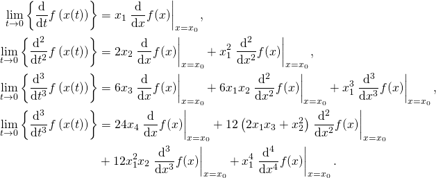
The right hand side is obtained by a repeated application of the chain rule. The first four derivatives are given by

$\begin{align*} \lim_{t \rightarrow 0} \left\{ \frac{\mathrm{d}}{\mathrm{d} t} f \left( x(t) \right) \right\} & = x_1 \left. \frac{\mathrm{d}}{\mathrm{d} x} f(x) \right|_{x = x_0},\\ \lim_{t \rightarrow 0} \left\{ \frac{\mathrm{d}^2}{\mathrm{d} t^2} f \left( x(t) \right) \right\} & = 2 x_2 \left. \frac{\mathrm{d}}{\mathrm{d} x} f(x) \right|_{x = x_0} + x_1^2 \left. \frac{\mathrm{d}^2}{\mathrm{d} x^2} f(x) \right|_{x = x_0},\\ \lim_{t \rightarrow 0} \left\{ \frac{\mathrm{d}^3}{\mathrm{d} t^3} f \left( x(t) \right) \right\} & = 6 x_3 \left. \frac{\mathrm{d}}{\mathrm{d} x} f(x) \right|_{x = x_0} + 6 x_1 x_2 \left. \frac{\mathrm{d}^2}{\mathrm{d} x^2} f(x) \right|_{x = x_0} + x_1^3 \left. \frac{\mathrm{d}^3}{\mathrm{d} x^3} f(x) \right|_{x = x_0},\\ \lim_{t \rightarrow 0} \left\{ \frac{\mathrm{d}^3}{\mathrm{d} t^3} f \left( x(t) \right) \right\} & = 24 x_4 \left. \frac{\mathrm{d}}{\mathrm{d} x} f(x) \right|_{x = x_0} + 12 \left( 2 x_1 x_3 + x_2^2 \right) \left. \frac{\mathrm{d}^2}{\mathrm{d} x^2} f(x) \right|_{x = x_0}\\ & + 12 x_1^2 x_2 \left. \frac{\mathrm{d}^3}{\mathrm{d} x^3} f(x) \right|_{x = x_0} + x_1^4 \left. \frac{\mathrm{d}^4}{\mathrm{d} x^4} f(x) \right|_{x = x_0}. \end{align*}$

The coefficients $x_n$ are weights on the derivatives that need to be passed to CppAD. That is, to compute the first order derivative, we set $x_1 = 1$ and get

$y_1 = \left. \frac{\mathrm{d}}{\mathrm{d} x} f(x) \right|_{x = x_0}.$

It is easy to show that in order to compute the $n$ -th order derivative, we set $x_1 = 1$ and $x_i = 0$ for $i = \{ 2, 3, \ldots, n \}$ to get

$n! y_n = \left. \frac{\mathrm{d}^n}{\mathrm{d} x^n} f(x) \right|_{x = x_0}.$

Code Example

In order to compute the $n$ -th order derivative in forward mode with CppAd, we first create an ADFun object which stores the operation sequence. We can then iteratively call .Forward(order, scalings) on this function to compute the vector $\bm{y} \in \mathrm{R}^{n + 1}$ for the coefficient vector $\bm{x} \in \mathrm{R}^{n + 1}$ .

// non-standard includes
#include <boost/container/small_vector.hpp>
#include <cppad/cppad.hpp>

// differentiate general function of one variable
template<size_t order, typename Type, typename Function>
small_vector<Type, order + 1> differentiate(Function function,
                                            Type xValue) {
    static_assert(order > 0, "Order has to be at least one.");

    // setup the mapping / record the sequence
    small_vector<AD<Type>, 1> xValue2 { xValue };
    Independent(xValue2);
    small_vector<AD<Type>, 1> yValue { function(xValue2[0]) };
    ADFun<Type> mapping(xValue2, yValue);

    // compute all orders at once
    small_vector<Type, order + 1> scalings(order + 1);
    scalings[0] = xValue;
    scalings[1] = Type(1.0);
    for (size_t i = 2; i <= order; ++i) {
        scalings[i] = Type(0.0);
    }
    auto result = mapping.Forward(order, scalings);

    // scale the results by the Taylor coefficients
    double multiplier = 1.0;
    for (size_t i = 2; i <= order; ++i) {
        multiplier *= static_cast<double>(i);
        result[i] *= multiplier;
    }
    return result;
}

Note that in the above code, we use small_vector form the Boost library instead of an STL vector to avoid heap allocations. While our previous discussion only considered real valued functions of a real variable, the function differentiate(...) has a templated parameter and return value type. Below is a simple test that differentiates a polynomial.

// general polynomial
template<size_t degreePlusOne, typename Type>
Type polynomial(array<double, degreePlusOne> const & coefficients,
                Type value) {
    Type result(coefficients[0]);
    Type power(1.0);
    for (size_t i = 1; i < degreePlusOne; ++i) {
        power *= value;
        result += power * coefficients[i];
    }
    return result;
}

int main() {
    // setup the test function
    array<double, 4> coefficients {{ 1.0, 1.0, 1.0, 1.0 }};
    auto function = [&](auto value) {
        return polynomial(coefficients, value);
    };

    // take the first four derivatives at x = 1.0
    auto derivatives = differentiate<4, double>(function, 1.0);
    for (size_t i = 0; i <= 4; ++i) {
        cout << i << " -> " << derivatives[i] << endl;
    }
}

In the above code, we can simply replace differentiate<4, double> by differentiate<4, complex>.

References

Homescu, Cristian (2011) “Adjoints and Automatic (Algorithmic) Differentiation in Computational Finance,” Working Paper, available at SSRN http://ssrn.com/abstract=1828503

Leave a Reply Cancel reply