Inverse Gaussian Ornstein-Uhlenbeck Stochastic Clocks - Matthias Thul's HomepageMatthias Thul's Homepage

In this pose, we consider an Ornstein-Uhlenbeck stochastic clock whose instantaneous rate of activity process has an inverse Gaussian stationary distribution. We use the previously obtained relationship between the cumulant generation function of the stationary distribution and that of the background driving Lévy process and show that the latter can be represented as the sum of an inverse Gaussian processes and a compound Poisson process with chi-squared distributed increments.

Related Posts

Construction via the Background Driving Lévy Process

We assume that the stationary distribution of $y$ is inverse Gaussian $\text{IG}(a, b)$ with characteristic exponent

$\psi_{y_\infty}(\omega) = -a \left( \sqrt{b^2 - 2 \mathrm{i} \omega} - b \right).$

This is the distribution of the first hitting time of a drifted Brownian motion $X_t = b t + W_t$ to the level $a > 0$ , where $b > 0$ ; see e.g. Schoutens (2003). As shown in a previous post, the following relationship holds

$\psi_{Z_1}(\omega) = \omega \psi_{y_\infty}'(\omega).$

Thus,

$\begin{align*} \psi_{Z_1}(\omega) = \frac{\mathrm{i} \omega a}{\sqrt{b^2 - 2 \mathrm{i} \omega}}. \end{align*}$

As shown by Barndorff-Nielsen (1998) we can decompose the background driving Lévy process as $Z_1 = Z_1^{(1)} + Z_1^{(2)}$ where $Z_1^{(1)} \sim \mathrm{IG} \left( a / 2, b \right)$ and

$Z_t^{(2)} = \frac{1}{b^2} \sum_{n = 1}^{N_t} X_i.$

Here $N = \left\{ N_t : t \in \mathbb{R}_{+, 0} \right\}$ is a Poisson process with arrival rate $a b / 2$ and $\left\{ X_i \right\}_{i = 1}^\infty$ is a sequence of independent identically distributed (i.i.d.) chi-squared $\chi_1^2$ random variables with degree of freedom one; see also Schoutens (2003). We have

$\psi_{Z_1^{(1)}}(\omega) = -\frac{a}{2} \left( \sqrt{b^2 - 2 \mathrm{i} \omega} - b \right).$

Next,

$\phi_X(\omega) = \frac{1}{\sqrt{1 - 2 \mathrm{i} \omega}}$

and thus

$\psi_{Z_1^{(2)}}(\omega) = \frac{a b}{2} \left( \phi_X \left( \frac{\omega}{b^2} \right) - 1 \right).$

Here, we used the general form of the characteristic function for compound Poisson processes. Summing the cumulant generating functions yields

$\psi_{Z_1^{(1)}}(\omega) + \psi_{Z_1^{(2)}}(\omega) = \frac{\mathrm{i} \omega a}{\sqrt{b^2 - 2 \mathrm{i} \omega}} = \psi_{Z_1}(\omega)$

as claimed.

Integrated Time-Change

We again start from the previously obtained general solution for the characteristic function of the total activity process $Y = \left\{ Y_t : \mathbb{R}_{+, 0} \right\}$ ,

$\phi_{Y_t}(\omega) = \exp \left\{ \frac{\mathrm{i} \omega y_0}{\lambda} \left( 1 - e^{-\lambda t} \right) + \lambda \int_0^t \psi_{Z_1} \left( \frac{\omega}{\lambda} \left( 1 - e^{\lambda (u - t)} \right) \right) \mathrm{d}u \right\}.$

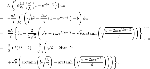
We evaluate the two integrals corresponding to $Z^{(1)}$ and $Z^{(2)}$ separately. The first one is

$\begin{eqnarray*} & & \lambda \int_0^t \psi_{Z_1}^{(1)} \left( \frac{\omega}{\lambda} \left( 1 - e^{\lambda (u - t)} \right) \right) \mathrm{d}u\\ & = & -\frac{a \lambda}{2} \int_0^t \left( \sqrt{b^2 - \frac{2 \mathrm{i} \omega}{\lambda} \left( 1 - e^{\lambda (u - t)} \right)} - b \right) \mathrm{d}u\\ & = & \left. \frac{a \lambda}{2} \left\{ b u - \frac{2}{\lambda \sqrt{\lambda}} \left( \sqrt{\theta + 2 \mathrm{i} \omega e^{\lambda (u - t)}} - \sqrt{\theta} \mathrm{arctanh} \left( \sqrt{\frac{\theta + 2 \mathrm{i} \omega e^{\lambda (u - t)}}{\theta}} \right) \right) \right\} \right|_{u = 0}^{u = t}\\ & = & \frac{a}{2} \left\{ b (\lambda t - 2) + \frac{2}{\sqrt{\lambda}} \Bigg( \sqrt{\theta + 2 \mathrm{i} \omega e^{-\lambda t}} \Bigg. \right.\\ & & \left. \left. + \sqrt{\theta} \left( \mathrm{arctanh} \left( b \sqrt{\frac{\lambda}{\theta}} \right) - \mathrm{arctanh} \left( \sqrt{\frac{\theta + 2 \mathrm{i} \omega e^{-\lambda t}}{\theta}} \right) \right) \right) \right\}. \end{eqnarray*}$

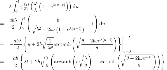
Here, we defined

$\theta = b^2 \lambda - 2 \mathrm{i} \omega.$

The second one is

$\begin{eqnarray*} & & \lambda \int_0^t \psi_{Z_1}^{(2)} \left( \frac{\omega}{\lambda} \left( 1 - e^{\lambda (u - t)} \right) \right) \mathrm{d}u\\ & = & \frac{a b \lambda}{2} \int_0^t \left( \frac{b}{\sqrt{b^2 - 2 \mathrm{i} \omega \left( 1 - e^{\lambda (u - t)} \right)}} - 1 \right) \mathrm{d}u\\ & = & \left. -\frac{a b \lambda}{2} \left\{ u + 2 b \sqrt{\frac{1}{\lambda \theta}} \mathrm{arctanh} \left( \sqrt{\frac{\theta + 2 \mathrm{i} \omega e^{\lambda (u - t)}}{\theta}} \right) \right\} \right|_{u = 0}^{u = t}\\ & = & -\frac{a b}{2} \left\{ \lambda t + 2 b \sqrt{\frac{\lambda}{\theta}} \left( \mathrm{arctanh} \left( b \sqrt{\frac{\lambda}{\theta}} \right) - \mathrm{arctanh} \left( \sqrt{\frac{\theta + 2 \mathrm{i} \omega e^{-\lambda t}}{\theta}} \right) \right) \right\}. \end{eqnarray*}$

Combining these two expressions and grouping terms yields

$\begin{eqnarray*} \phi_{Y_t}(\omega) & = & \frac{\mathrm{i} \omega y_0}{\lambda} \left( 1 - e^{-\lambda t} \right) + a \left\{ \sqrt{\frac{\theta + 2 \mathrm{i} \omega e^{-\lambda t}}{\lambda}} - b \right.\\ & & \left. -\frac{2 \mathrm{i} \omega}{\sqrt{\lambda \theta}} \left( \mathrm{arctanh} \left( b \sqrt{\frac{\lambda}{\theta}} \right) - \mathrm{arctanh} \left( \sqrt{\frac{\theta + 2 \mathrm{i} \omega e^{-\lambda t}}{\theta}} \right) \right) \right\}. \end{eqnarray*}$

This expression coincides with the one given in Schoutens (2003), who defines

$\kappa = \frac{\theta}{b^2 \lambda} - 1$

instead.

References

Barndorff-Nielsen, Ole E. (1998) “Processes of Normal Inverse Gaussian Type”, Finance and Stochastics, Vol. 2, No. 1, pp. 41-68

Schotens, Wim (2003) Lévy Processes in Finance: John Wiley & Sons

Leave a Reply Cancel reply